OptiNod Academy
TradingView backtesting — from initial settings to CSV analysis
Apply a strategy, set capital, fees, slippage and dates, diagnose zero trades, read results and analyze the trade CSV. Keep the conditions so the next test is comparable.
Your first backtest is a run with its settings and trade records saved. Those conditions make the next result comparable.
A strategy may produce no trades, or its profit may disappear when fees are added. Start with the rule that creates each order and the size it uses.
TradingView backtesting applies trading rules to historical data to produce simulated trades. Buy and sell markers, live fills and simulated report trades are separate records.
Follow this sequence: apply a strategy → set costs and dates → inspect the first trade → read results → save the trade list. Then analyze the CSV in OptiNod and use the loss-making trades to plan the next check.
Apply a strategy to see orders and results together
Start with a standard candlestick chart. Choose the exchange-qualified symbol and timeframe. Add a strategy you are permitted to use, and record its name, source version and inputs. Adding an indicator such as a moving average does not create backtest trades. A strategy needs a strategy() declaration and commands that place simulated orders.
Current official documentation calls the panel below the chart Strategy report and its result tabs Metrics and Trades. Depending on language and interface version, you may see older labels such as Strategy Tester, Overview and List of Trades. Find both the trade list and the performance metrics in your interface. Official strategy documentation
Starting with standard candles reduces the chance of mixing synthetic chart prices into the fill assumptions. After adding the strategy, look for actual entry and exit records.
The example is OptiNod Learn - SMA 10/30 Backtest Guide v1.0.0. We selected NASDAQ:AAPL, standard candles and 1D; the screen feed was labeled NASDAQ by Cboe One. It was checked on 2026-10-01. This original educational script enters long when SMA 10 crosses above SMA 30 and closes when it crosses below. It has no separate stop, profit target or live-trading alerts, and is not a performance recommendation.
- Open a new script in TradingView's Pine Editor and paste the code below.
- Apply it to the chart and match NASDAQ:AAPL, 1D and standard candles.
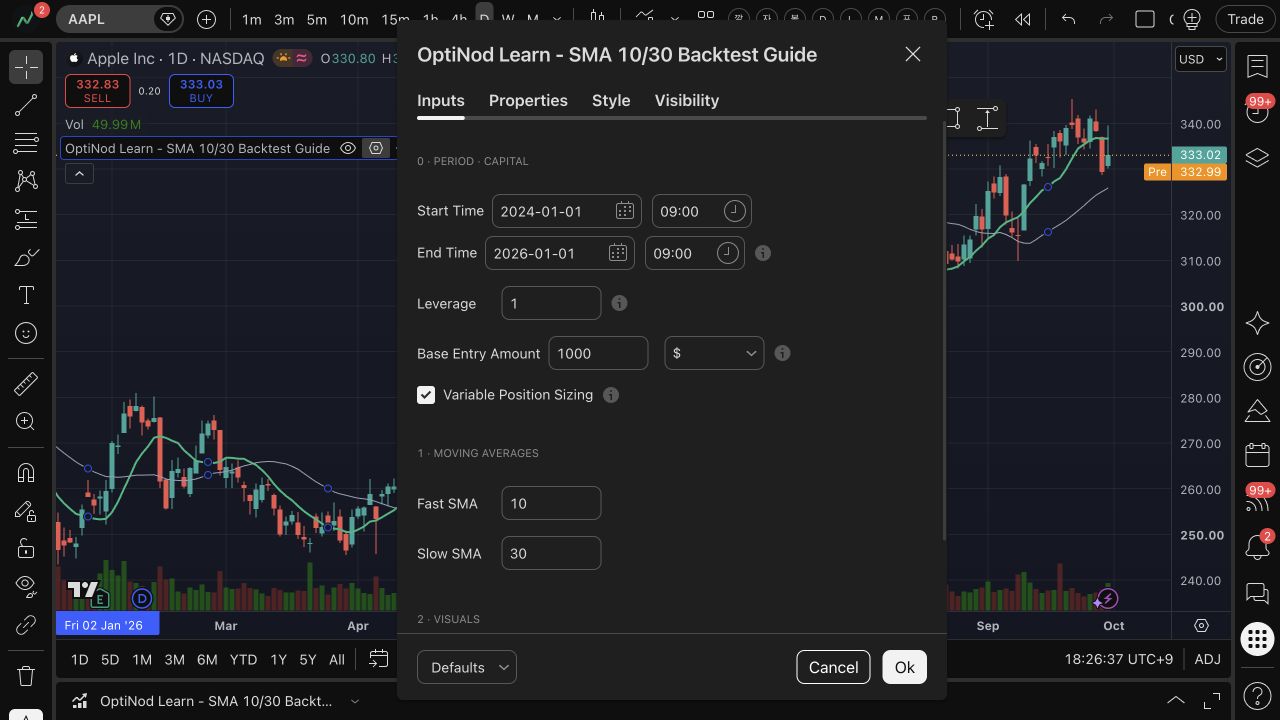
- Compare dates and Base Entry Amount in Inputs, then capital, costs and fill settings in Properties.
- Open the trade list and metrics and compare with the observed results below under the same conditions.
//@version=6
// OptiNod Learn educational example v1.0.0. AAPL standard candles, 1D.
// Simulated orders only. No alerts or webhook payloads are defined.
strategy("OptiNod Learn - SMA 10/30 Backtest Guide", overlay=true, pyramiding=0, initial_capital=10000, currency=currency.USD, default_qty_type=strategy.fixed, default_qty_value=1, commission_type=strategy.commission.percent, commission_value=0.05, slippage=1, margin_long=100, margin_short=100, process_orders_on_close=false, calc_on_every_tick=false, calc_on_order_fills=false, use_bar_magnifier=false)

// 0 - Period / Capital: first input group, before signal and visual inputs.
string G_CAP = "0 · Period · Capital"
int startTime = input.time(1704067200000, "Start Time", group=G_CAP, inline="win") // 2024-01-01 00:00 UTC
int endTime = input.time(1767225600000, "End Time", group=G_CAP, inline="win", tooltip="Entries use bar opening times in [start, end). An open position is closed at the first calculated bar at or after end; market fills normally occur on the next available tick.") // 2026-01-01 00:00 UTC
float leverage = input.float(1.0, "Leverage", minval=1.0, maxval=1.0, step=1.0, group=G_CAP, tooltip="This educational stock example is unleveraged: 1x only. Margin requirement is 100%.")
float baseAmount = input.float(1000.0, "Base Entry Amount", minval=0.0, group=G_CAP, inline="amt")
string amountUnit = input.string("$", "", options=["%", "$"], group=G_CAP, inline="amt", tooltip="Margin budget per entry in USD. % uses current strategy equity; $ uses a fixed amount. Whole-share rounding makes actual exposure no greater than the budget at the signal close.")
bool useVarSizing = input.bool(true, "Variable Position Sizing", group=G_CAP, tooltip="The standard header keeps this control. This simple example always uses multiplier 1, so toggling it does not change sizing.")

string G_SIGNAL = "1 · Moving Averages"
int fastLength = input.int(10, "Fast SMA", minval=1, group=G_SIGNAL)
int slowLength = input.int(30, "Slow SMA", minval=1, group=G_SIGNAL)

string G_VIEW = "2 · Visuals"
bool showAverages = input.bool(true, "Show averages", group=G_VIEW)
color fastColor = input.color(#10b981, "Fast", group=G_VIEW, inline="palette")
color slowColor = input.color(#9aa0b5, "Slow", group=G_VIEW, inline="palette")

// AAPL whole shares. Quantity uses the signal close, not an unknowable future fill.
qtyFor(float stateMult) =>
    float margin = (amountUnit == "%" ? strategy.equity * baseAmount / 100.0 : baseAmount) * (useVarSizing ? stateMult : 1.0)
    math.floor(math.max(margin, 0.0) * leverage / (close * syminfo.pointvalue))

bool inWindow = time >= startTime and time < endTime
float fastSma = ta.sma(close, fastLength)
float slowSma = ta.sma(close, slowLength)
bool longSignal = ta.crossover(fastSma, slowSma)
bool exitSignal = ta.crossunder(fastSma, slowSma)
float entryQty = qtyFor(1.0)

if inWindow and longSignal and strategy.position_size == 0 and entryQty > 0
    strategy.entry("Long", strategy.long, qty=entryQty, comment="Long")

if strategy.position_size > 0 and time >= endTime
    strategy.close("Long", comment="Time exit")
else if strategy.position_size > 0 and exitSignal
    strategy.close("Long", comment="Exit")

// Layout: Minimal Overlay. Two averages explain the educational crossover.
plot(showAverages ? fastSma : na, "Fast SMA", color=fastColor, linewidth=2)
plot(showAverages ? slowSma : na, "Slow SMA", color=slowColor, linewidth=1)
Quantity is a 1,000 USD budget divided by the signal close and rounded down to whole shares. It is not an order whose actual fill value is exactly 1,000 USD. Next-bar gaps and slippage can change the filled notional. Leverage is fixed at 1x. Variable Position Sizing is enabled, but its multiplier is always 1, so the toggle does not change quantity.
Set costs and size before comparing runs
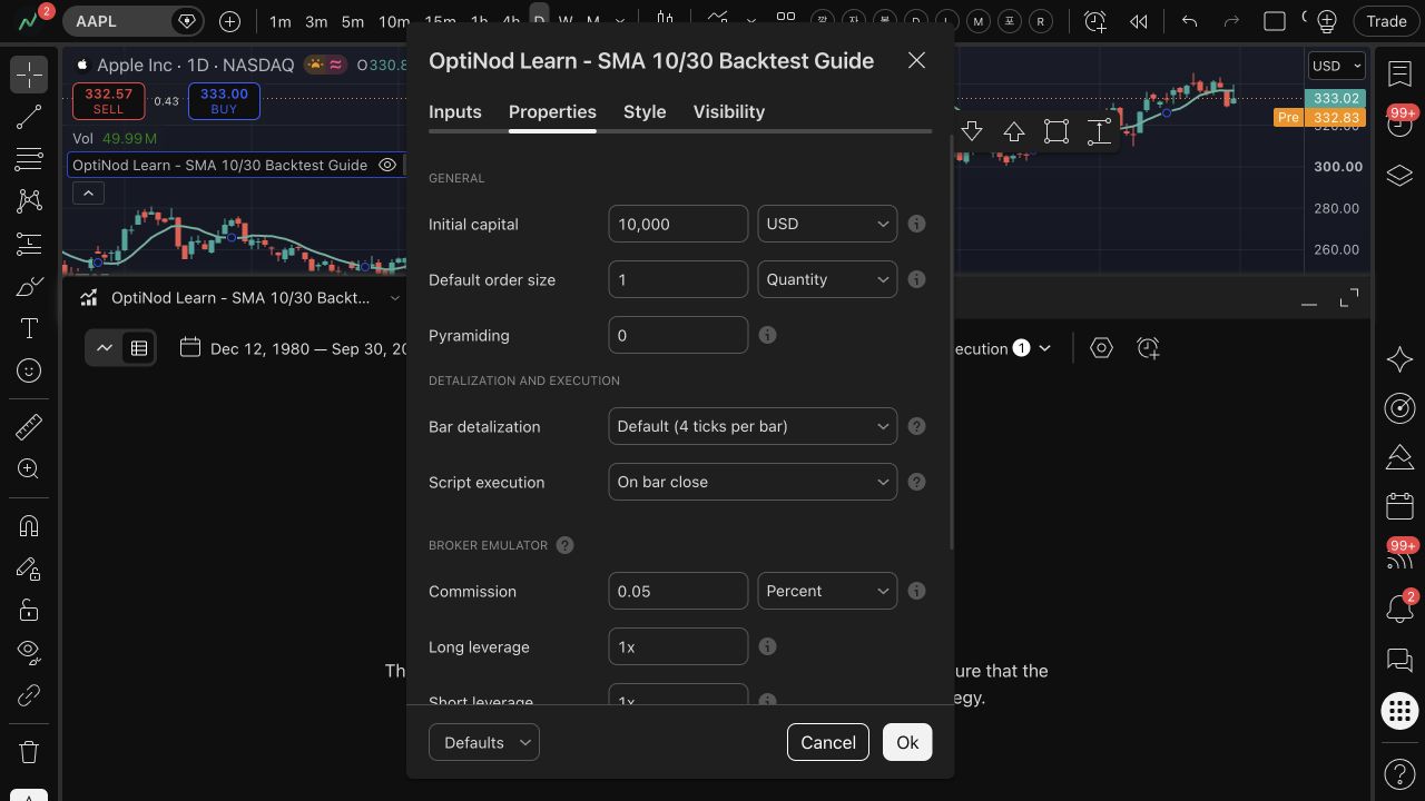
Open the strategy settings, then Properties, and set capital, order size, commission and slippage. The table records the settings and units used in the observed run.
| Setting | Value actually used | Unit | Why it affects results |
|---|---|---|---|
| Initial capital/currency | 10,000 USD | USD | Starting equity and return reference |
| Base Entry Amount | 1,000, unit $ | USD/entry budget | Code calculates whole shares at the signal close |
| Leverage/margin | 1x; long and short margin 100% | multiplier, % | Unleveraged simulated orders within available capital |
| Commission | 0.05 | %/order | 0.05% of each entry and exit transaction |
| Slippage | 1 | tick | Applied to market and stop fill prices |
| Bar detail | Default (4 ticks per bar) | 4 price points/bar | Default OHLC assumptions for historical fills |
| Script execution | On bar close | bar close | Crossovers are calculated when the bar closes |
| Order execution delay | One tick | 1 tick | Market orders fill on the next available tick |
The price adjustment is ticks × the symbol's minimum tick size. Equity-percentage sizing changes the amount with equity at entry. If the code assigns a quantity to an individual order, changing the default size may not change that order. Official property definitions
Also record margin, recalculation and fill options. Keep the effects of cost and position size separate from changes to the trading rules.
Properties showed a default order size of 1, but this script passes qty directly to strategy.entry(). Actual quantity comes from Base Entry Amount in Inputs. Compare Default detalization and Script execution in the report with Properties in strategy settings.
Read dates alongside the available chart data
A regular backtest runs on data loaded on the chart. A strategy's date input restricts orders within that data; it does not load older history. If date inputs are available, set the start and end and compare actual trade timestamps with the intended period.
Testing period selection and Deep Backtesting are separate features. Record what your account supports and the result period shown on screen. Do not assume every account offers a period selector. Dates and chart-data guidance
Record the display timezone, exchange session, first available bar and calculation warm-up as well. Matching date inputs alone does not establish identical datasets.
The observed Inputs were 2024-01-01 00:00 UTC to 2026-01-01 00:00 UTC. On the Korean-time screen they appeared as 09:00. New orders are created only when the signal bar's opening time is at or after the start and before the end.
The report calculation range was 1980-12-12–2026-09-30, which differs from the entry window limited by the script. The first actual entry was 2024-01-30 and the last close 2025-12-23. Earlier loaded bars are used for warm-up; the report range is not the entry window.
If a position remains after the end, the script requests a close on the first calculated bar at or after that time, with execution on the next available tick. It does not liquidate at the exact end timestamp. An entry order created inside the window can also fill outside it on the next bar.
With zero trades, narrow down the order path first
Check that the script is a strategy and contains order commands. If the chart shows a runtime error marker, open it and read the message. Then check the overlap between the date filter and chart data, and whether an entry condition occurred.
Zero order size or insufficient capital and margin for the requested size can prevent trades. A futures contract's value depends on point value and quantity, so chart price alone does not establish affordability.
Zero-trade check: script type and runtime errors → data and dates → entry conditions → order size and capital. Change one setting at a time and see whether a trade appears. Once it does, compare entry and exit times, prices, size and signals with the chart.
Use why a strategy generates no orders to narrow down the cause before reading performance. A run with no trades and a run with losses require different next actions.
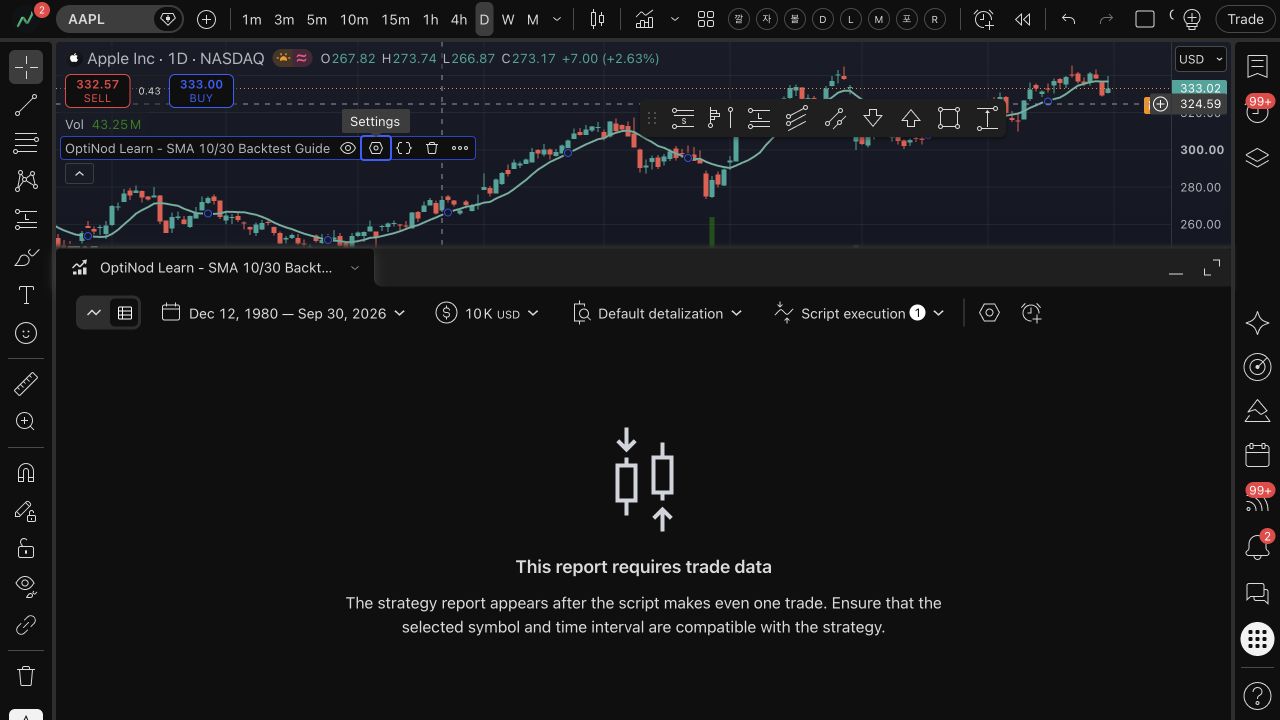
Setting both Fast SMA and Slow SMA to 10 actually produced “This report requires trade data”. Identical averages do not cross each other, so the order condition never occurred. Restore Slow SMA to 30 to return to the original 10/30 crossover. This was an unmet-condition case; increasing capital would not fix it.
After net PnL, return to the losing trades
Net PnL already includes configured commission. Subtracting Commission paid again counts the fees twice. Read Open PnL separately from realized trade results. Commission handling
| Metric | Reading basis | What it cannot establish alone |
|---|---|---|
| Closed trades | Count trades that entered and closed | Whether future trade frequency will match |
| PF | Sum of winning PnL ÷ absolute sum of losing PnL | Whether profits depend on a few trades or periods |
| Expected payoff | Net PnL ÷ closed-trade count | Outcome distribution and the size of large losses |
| Maximum drawdown | Record intrabar/close-to-close basis and percentage denominator | Whether future drawdown will stay within that range |
Total trades, PF and expected payoff exclude open positions. A zero loss sum does not yield a finite PF for ordinary comparison. Rather than impose a universal passing PF or minimum trade count, inspect timing and outcome distribution.
Intrabar maximum drawdown includes price movement within bars while positions are open. It may differ from drawdown calculated only from cumulative closed-trade PnL. Distinguish a percentage of initial capital from percentages with other denominators. Read intrabar drawdown and drawdown relative to initial capital, then open the chart around the largest losses.
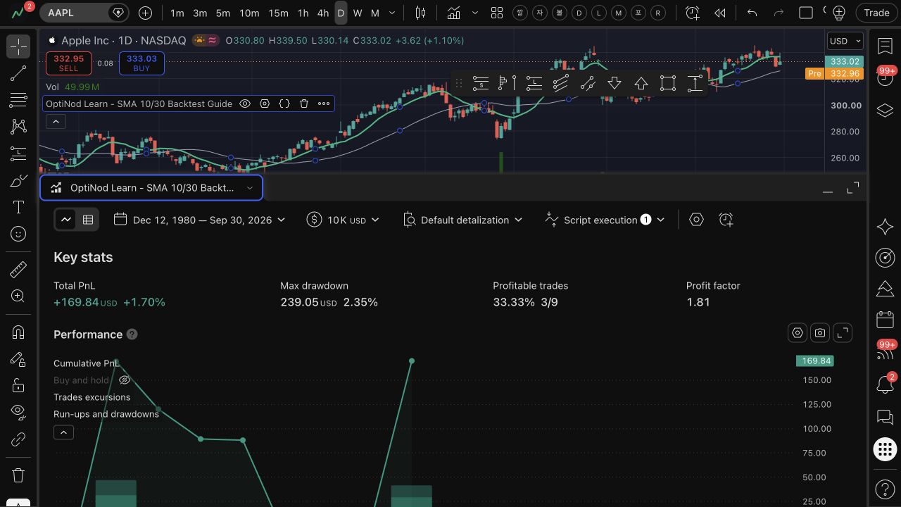
We compared the TradingView run with its English trade-list CSV. There were 18 entry/exit rows and 9 closed trades. Both rows repeat the trade PnL, so the reconciliation uses exit rows only.
| Item | Observed example | Meaning | What it cannot establish alone |
|---|---|---|---|
| Closed trades | 9; 3 winners and 6 losers | Completed-trade sample | Future frequency and repeatability |
| Total PnL | 169.84 USD, +1.70% | Matches the sum of exit-row net PnL | Whether another period produces the same outcome |
| Profit factor | Screen 1.81; CSV about 1.81015 | Reconciled as 379.48 ÷ 209.64 | Dependence on a small number of winners |
| Expectancy | 18.87 USD | 169.84 ÷ 9 ≈ 18.87111 | Individual loss sizes and outcome distribution |
| Max drawdown | Screen 239.05 USD, 2.35% | Maximum drawdown under that TradingView calculation | Whether the intrabar path can be reconstructed from CSV |
The exit PnL sum is 169.84 USD. Winning PnL totals 379.48 USD and absolute losing PnL 209.64 USD, based on rounded CSV fields. The TradingView aggregate loss display was 209.63 USD, a 0.01 USD difference; sums of rounded rows can differ slightly from the internal aggregate display.
Do not describe the displayed 2.35% as 239.05 ÷ 10,000: that calculation is about 2.3905%. Keep the drawdown metric's calculation basis distinct. The return +1.70% does match 169.84 ÷ 10,000 × 100 = 1.6984%, rounded.
Import the trade-list CSV to revisit loss periods
Save the CSV using Download in Trades or List of Trades. Metric exports and trade-list exports contain different information. Even if a complete XLSX report is available, the OptiNod input used here is the trade-list CSV. Official export guidance
Open the file and look for trade numbers, entry/exit timestamps and net PnL. Keep its filename alongside the strategy, symbol, timeframe and settings. Counting every entry and exit row can differ from counting completed trades.
Upload the trade-list CSV to OptiNod analysis, then compare closed-trade count and net PnL with the original report first. Trade lists with Korean or English headers are supported. If another language is not recognized, change TradingView's display language to Korean or English and export again. A file containing only open trades cannot produce closed-trade analysis.
You can begin analysis without signing in; saving it to an account requires sign-in or registration. Find the trades and periods contributing to losses, then return to their charts and conditions. CSV-based drawdown does not exactly reconstruct the original intrabar maximum drawdown, so read its calculation basis.
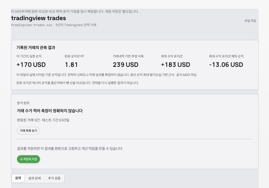
We imported the English CSV's 18 rows directly into OptiNod and confirmed that analysis opened. Completed positions showed 9, realized PnL 170 USD and PF 1.81. The 170 USD display rounds 169.84 USD. The first trade showed entry 2024-01-30, exit 2024-02-12 and PnL -13.65 USD.
OptiNod's 239 USD is explicitly labeled estimated drawdown from trade records. Similar rounded values do not mean that TradingView's official 239.05 USD intrabar MDD was exactly reconstructed. Open this first loss in the trade list and compare its entry, exit and costs with the original chart.
Separate the condition you change from the conditions you keep
To compare costs, keep source, inputs, symbol, timeframe, dates and order size fixed. To compare periods, keep rules and costs fixed while changing dates. Splitting one file chronologically is different from rerunning the strategy on a new data period.
Continue with slippage, fees and liquidity for costs and fills, lookahead and repainting for signal timing, and overfitting for stability around chosen settings. Walk-forward analysis covers repeating the procedure on periods not used for optimization; backtest versus live covers the first divergence from actual trading.
When saving the next run, write one line describing what changed. Preserved conditions and trade records let you return to the trades that caused the difference.